
Polynomial Regression in Machine Learning: Complete Guide 2026
Updated: 26 May 2026, 5:05 pm IST
According to the recent data by Gartner, total spending on AI is expected to reach $2.59 trillion by the end of 2026. This figure highlights the importance of applying data analytics and machine learning skills with multiple model applications in reality. Polynomial regression in machine learning is one of them.
Real-world business data is not perfectly linear; it has multiple curves. Just as sales demand changes seasonally, customer growth accelerates and slows down. These significant changes affect pricing trends, creating a fluctuation over time. In such cases, the traditional linear regression concept fails to capture real-world patterns accurately.
This is where the data analysts use polynomial regression. This guide provides a clear concept of what polynomial regression is, how it works, how it is different from linear regression and other important aspects.
What is Polynomial Regression?
Polynomial regression definition in machine learning denotes a concept of a supervised machine learning algorithm used to ensure non-linear relationships between variables. The model extends linear regression by transforming certain input features into existing polynomial terms. Thus, it allows the model to fit different curved patterns within the data.
On the other hand, in simple terms, polynomial regression helps in machine learning models when the relationship between variables is not linear. In simple terms, the model shows curves signalling the changed patterns of a business in multiple aspects.
For example:
- Advertising spend vs sales growth
- Temperature vs electricity consumption
- Product pricing vs customer demand
These relationships usually form curves rather than working with linear trends.
Also Read: A Complete Machine Learning Roadmap for Beginners
Polynomial Regression Formula in Machine Learning
The polynomial regression formula in machine learning shows a non-linear relationship between the independent variable x and dependent variable y.
y = β₀ + β₁x + β₂x² + β₃x³ + ... + βₙxⁿ + ε
These denotes:
- y = dependent variable
- x = independent variable
- β = regression coefficients
- n = polynomial degree
- ε = error term
One important technical point: even though the relationship between y and x is non-linear (curved), the relationship between y and the coefficients is still linear. That is why you can use standard linear regression methods after transforming the features.
Also Read: Types of Machine Learning You Should Know About

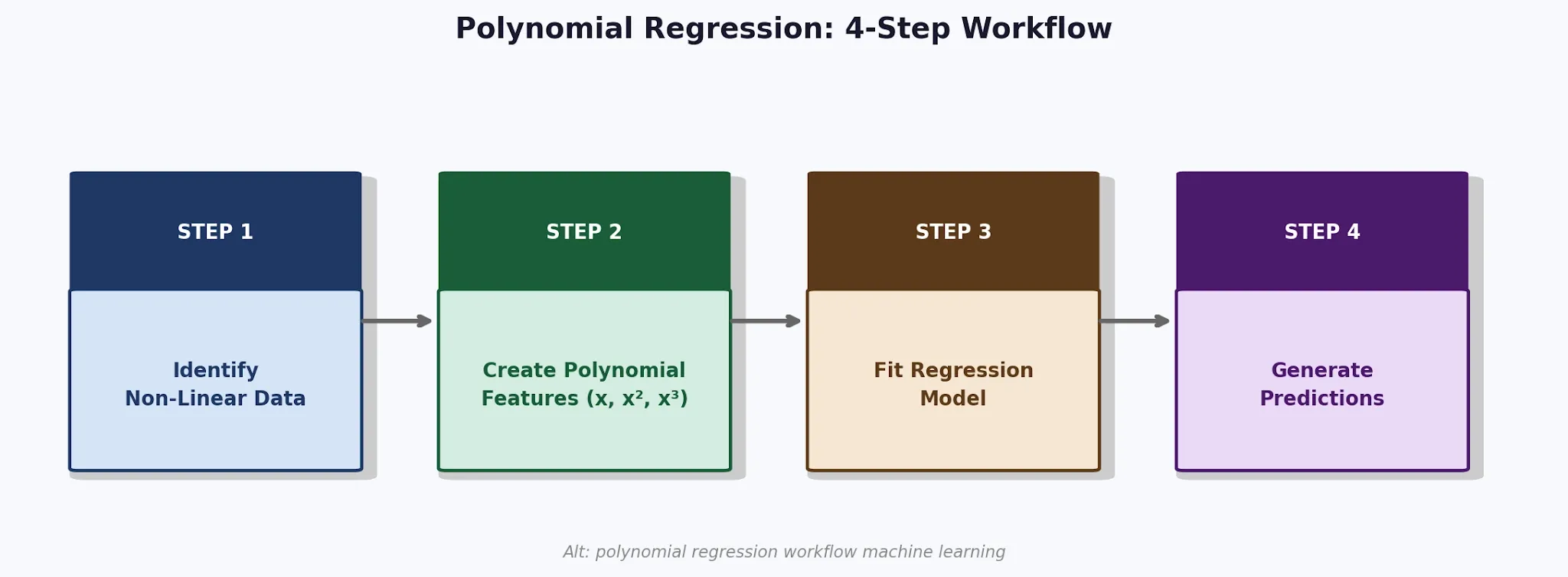
How Polynomial Regression Works
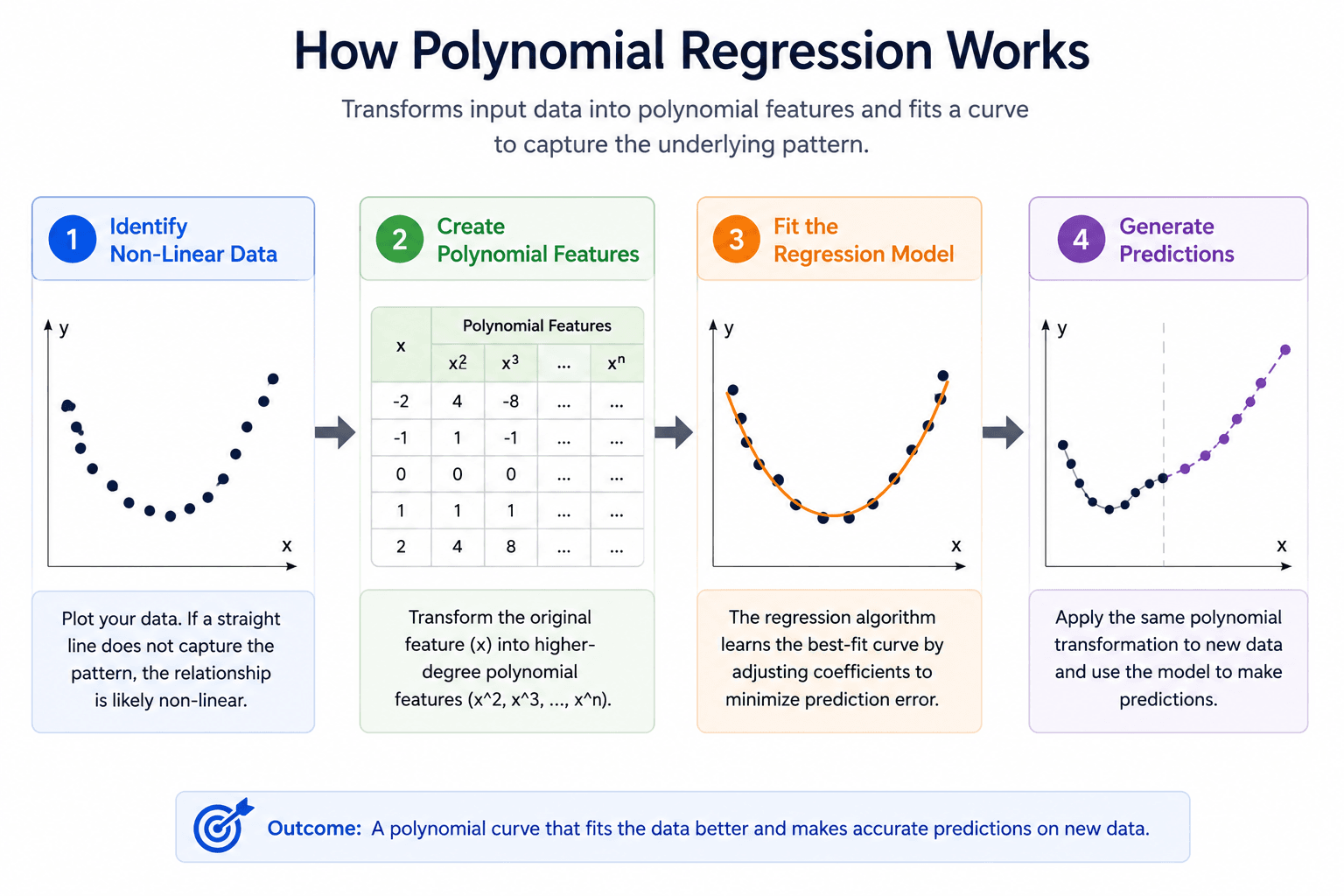
Polynomial regression in ML works by transforming original input variables into higher-degree polynomial features. Instead of being integrated into a straight line, the algorithm fits a curve and shows an accurate graph showing the variables.
Step 1: Identify Non-Linear Data
Plot your data before choosing a model. If a straight line clearly misses the pattern or curves upward, flattens, or reverses direction, the linear regression shows underfit. That is the signal that you should use polynomial regression.
Step 2: Create Polynomial Features
The original input feature x transforms into higher-order terms. Degree 2 develops x and x². Degree 3 develops x, x², and x³. This transformation is known as polynomial feature engineering, where each of the models shows flexibility and fit according to the curves.
Step 3: Fit the Regression Model
A linear regression algorithm calculates the best-fit curve by transforming certain features. The model also adjusts coefficients to minimise the chances of prediction error across the training data.
Step 4: Generate Predictions
The trained model applies learned coefficients to new data. The same polynomial transformation that was used during training models must also be applied to new data before prediction. However, skipping this step can cause some common implementation mistakes.
A Business Example:
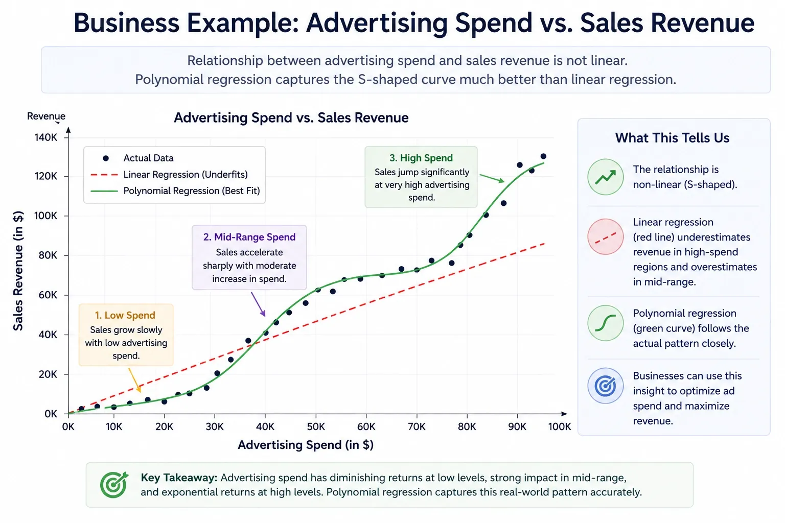
Consider a scenario for business, such as an advertising spend vs. sales revenue. Suppose a business spends little on advertising. It gives slow growth. When they opt for a mid-range spend, it accelerates the sales sharply. Similarly, a very high spend increases the revenue.
This advertising spend pattern (denoted as S) shows the changes in a business’s sales pattern and how it impacts its growth curve.
The S-shaped curve in the image shows exactly what polynomial regression captures and what linear regression misses entirely.
Also Read: Machine Learning Guide: Importance & Benefits
What is a Degree and Why Does It Matter in Polynomial Regression?
The concept of degree in a polynomial is the single most important decision you make when using this method. It controls how many bends and turns the fitted curve can have.
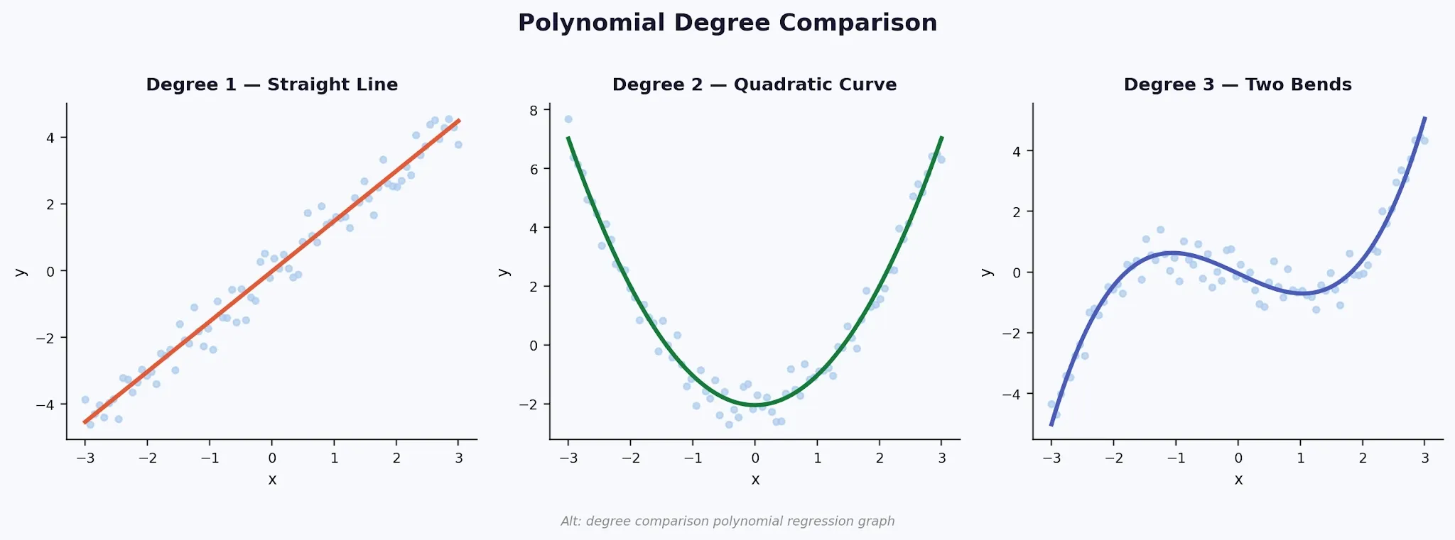
1. Degree 1
It is just linear regression. One straight line. Appropriate only when your data genuinely follows a straight trend.
2. Degree 2 (Quadratic)
gives you a U-shape or an inverted U. This fits data that rises and then falls, or falls and then rises. Think of how sales respond to price; they hold steady at moderate prices, then drop sharply at extremes. A quadratic curve handles that naturally.
3. Degrees 3 and above
add more bends. Degree 3 allows two direction changes. Higher degrees add further complexity. They become necessary for patterns with multiple peaks and troughs, but they come with serious risks, more on that shortly.
Here’s a quick table that might provide a clear overview.
| Degree | Curve Shape | When to Use |
|---|---|---|
| 1 | Straight line | Purely linear data |
| 2 | U-shaped parabola | Single curve or inflexion |
| 3 | Two bends | Two direction changes |
| 4+ | Multi-bend | Highly complex patterns |
Polynomial Regression vs Linear Regression: What Actually Differs
While practically working on the Polynomial regression curve, many candidates often ask whether they should just always use polynomial regression since it is more flexible.
The answer is no; rather, you should understand where it differs from linear progression. Having a clear concept of this can help you to analyse the data better. Here’s a table showing the overview of this.
| Key Features | Polynomial Regression | Linear Regression |
|---|---|---|
| Relationship type | Linear | Non-linear |
| Curve shape | Straight Line | Curved |
| Complexity | Low | Moderate to high |
| Flexibility | Limited | High |
| Overfitting Risk | Lower | Higher with a large degree |
| Best Use Case | Simple linear datasets | Curved or complex datasets |
Linear regression often fails when the variable relationship is curved. A systematic pattern in residuals rather than random scatter signals that polynomial regression is needed.
Polynomial regression performs better when data shows visible curves, when linear models show clear underfitting, or when domain knowledge confirms non-linearity.
Also Read: Types of Machine Learning: A Beginner's Guide
Polynomial Feature Transformation in Machine Learning
Polynomial regression transforms certain input features before fitting the model. The regression method itself does not change, but the input data structure does.
| Original Feature | Degree 2 Feature | Degree 3 Features |
|---|---|---|
| x | x, x² | x, x², x³ |
| x₁, x₂ | x₁, x₂, x₁², x₂², x₁x₂ | Adds x₁³, x₂³, cross-terms |
This is one of the core features of machine learning models and data engineering. As the degree increases, the feature count grows quickly. However, with multiple input variables, this increases the chances of dimensionality and can also slow down training.
In Python, scikit-learn automates this with PolynomialFeatures. This creates all transformed columns before the regression model is fully trained.
This transformation increases job scopes for data analysts. According to the U.S. Bureau of Labor Statistics, data scientist jobs are predicted to grow by 34% between 2024 and 2034, much faster than the average for most occupations.
Also Read: Regression in Machine Learning: Types & Examples
Polynomial Regression Implementation in Python Using Scikit-learn
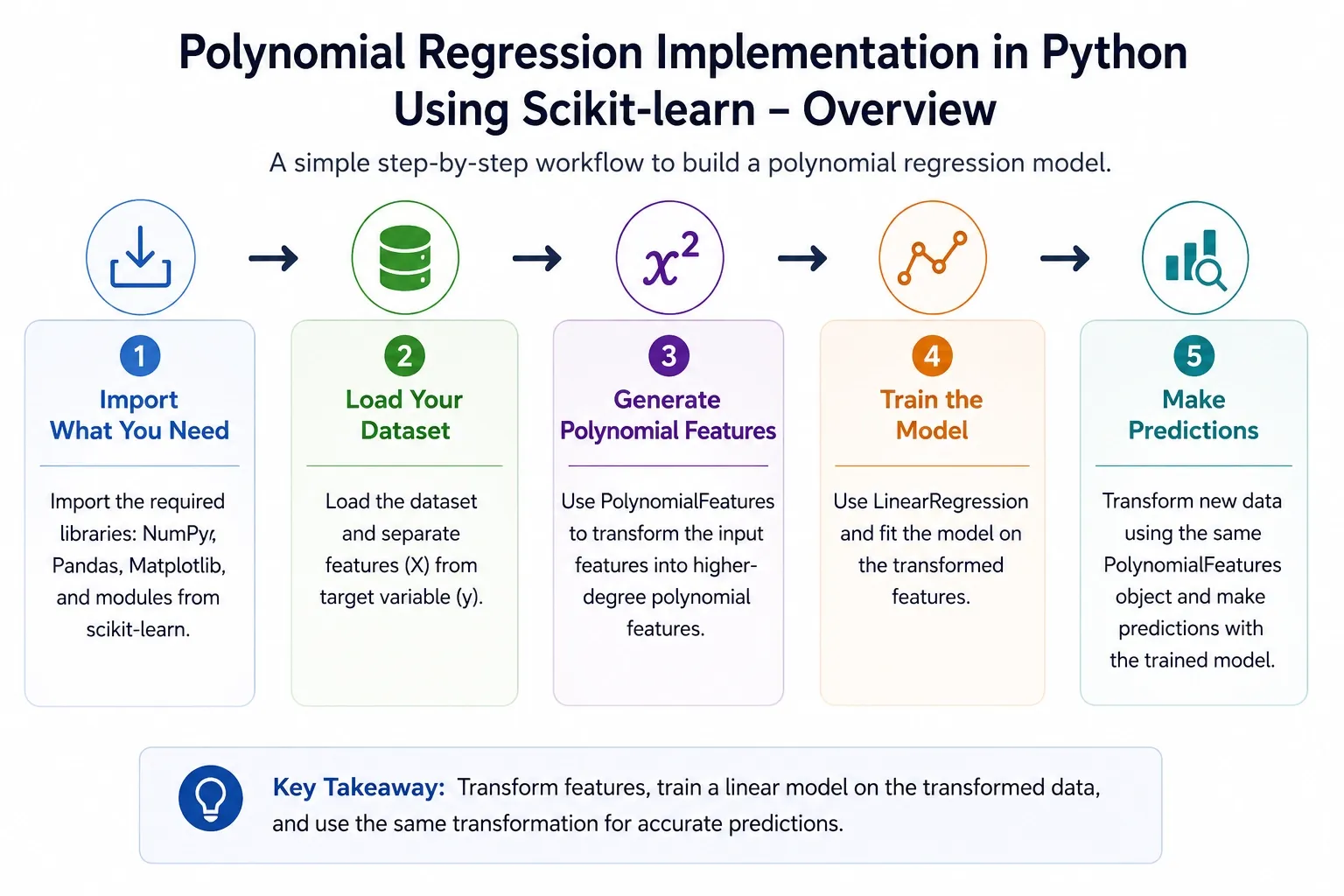
Polynomial regression method follows an implementation process in Python. Though it is a complex one, using scikit-learn can make this easy and straightforward. Here is the conceptual flow for a clear insight:
1. Import What You Need
NumPy for numerical operations, Pandas for tabular data, Matplotlib for visualisation, and scikit-learn for feature transformation and the regression model itself.
2. Load Your Dataset
Separate feature columns from the target column. For practice, a synthetic dataset with a visible curve works well.
3. Generate Polynomial Features
Import PolynomialFeatures from sklearn.preprocessing, set your degree, and call fit_transform() on your input data. This produces the expanded feature matrix.
4. Train the Model
Import LinearRegression from sklearn.linear_model and call fit() on the transformed features. The algorithm learns optimal coefficients.
5. Make Predictions
Call predict() on transformed test data. The test data must pass through the same PolynomialFeatures object used during training; skipping this step produces entirely wrong results.
The main key functions are: PolynomialFeatures(), LinearRegression(), fit_transform(), fit(), predict().
Also Read: AI Machine Learning Courses 2026: Complete Career Guide
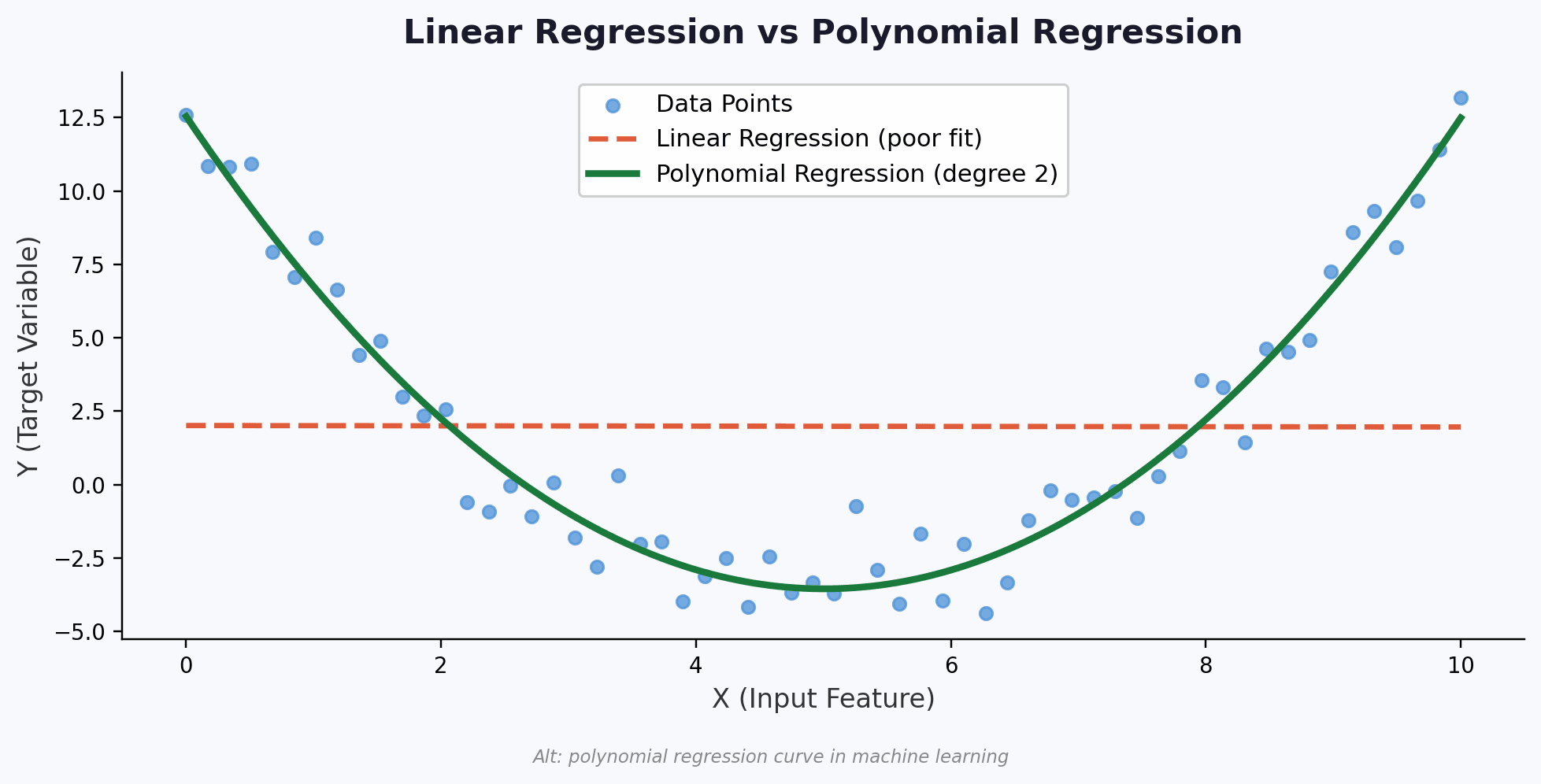
Visualising Polynomial Regression Curves
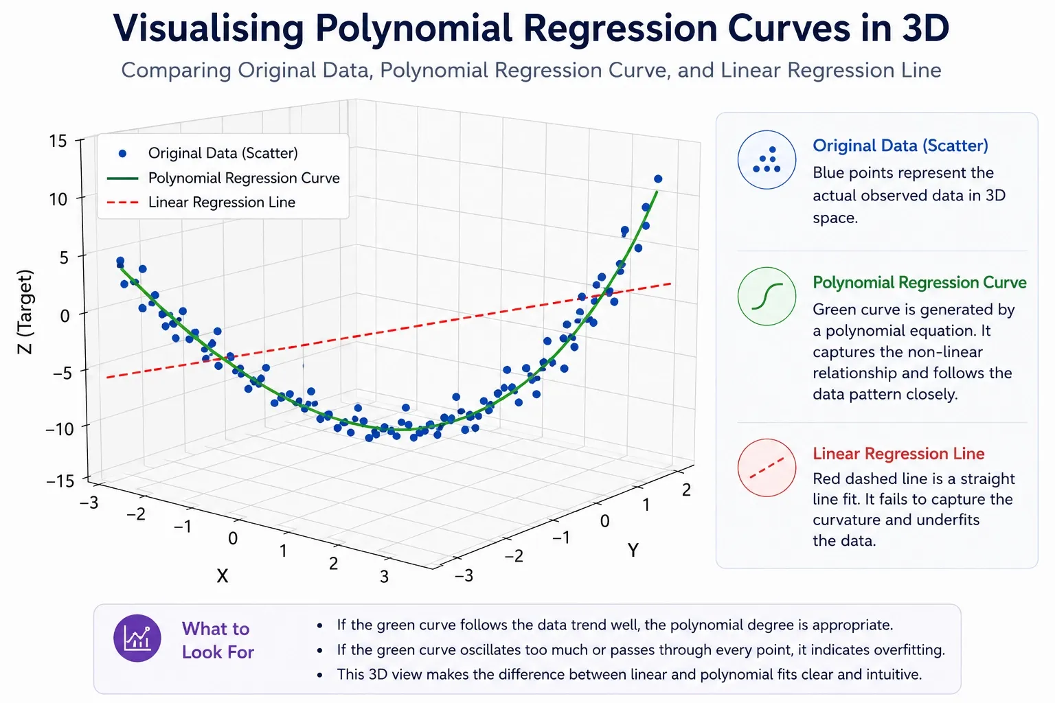
Visuals in Polynomial regression curves actually help to understand the original data and scattered plots, overlaying the curves generated by the Polynomial equation.
Use three-dimensional plotting in Python using Matplotlib. Build a three-layer plot scatter points from the original data, the polynomial regression curve as a smooth line, and a straight linear regression line alongside it for direct comparison.
The contrast makes the model value immediately clear. The curved line follows the data; the straight line misses it. If your curve oscillates wildly or passes through every single training point, that is a visual sign of overfitting.
Step-by-Step Polynomial Regression Mathematical Example
To understand the concept of polynomial regression method Polynomial regression clearly, here is a step-by-step mathematical example you can consider.
1. Identify Non-Linear Relationships
This is the first step where you can recognise that linear regression is actually underfitting the data.
For example:
- A straight line cannot model each of the seasonal sales patterns accurately. Hence, it creates curves in the chart showing the differences.
- Customer acquisition costs may rise exponentially after reaching to a certain threshold.
2. Transform Features into Polynomial Terms
In this step, the model generates some additional features such as:
- x²
- x³
- x⁴
These transformed features help the algorithm capture the curvature.
3. Train the Regression Model
The algorithm in the regression model considers multiple parameters. Train it accordingly, so it calculates after proper optimisation. It minimises prediction error.
4. Generate Predictions
Once trained, the model predicts outputs using the fitted polynomial curve.
Overfitting in Polynomial Regression
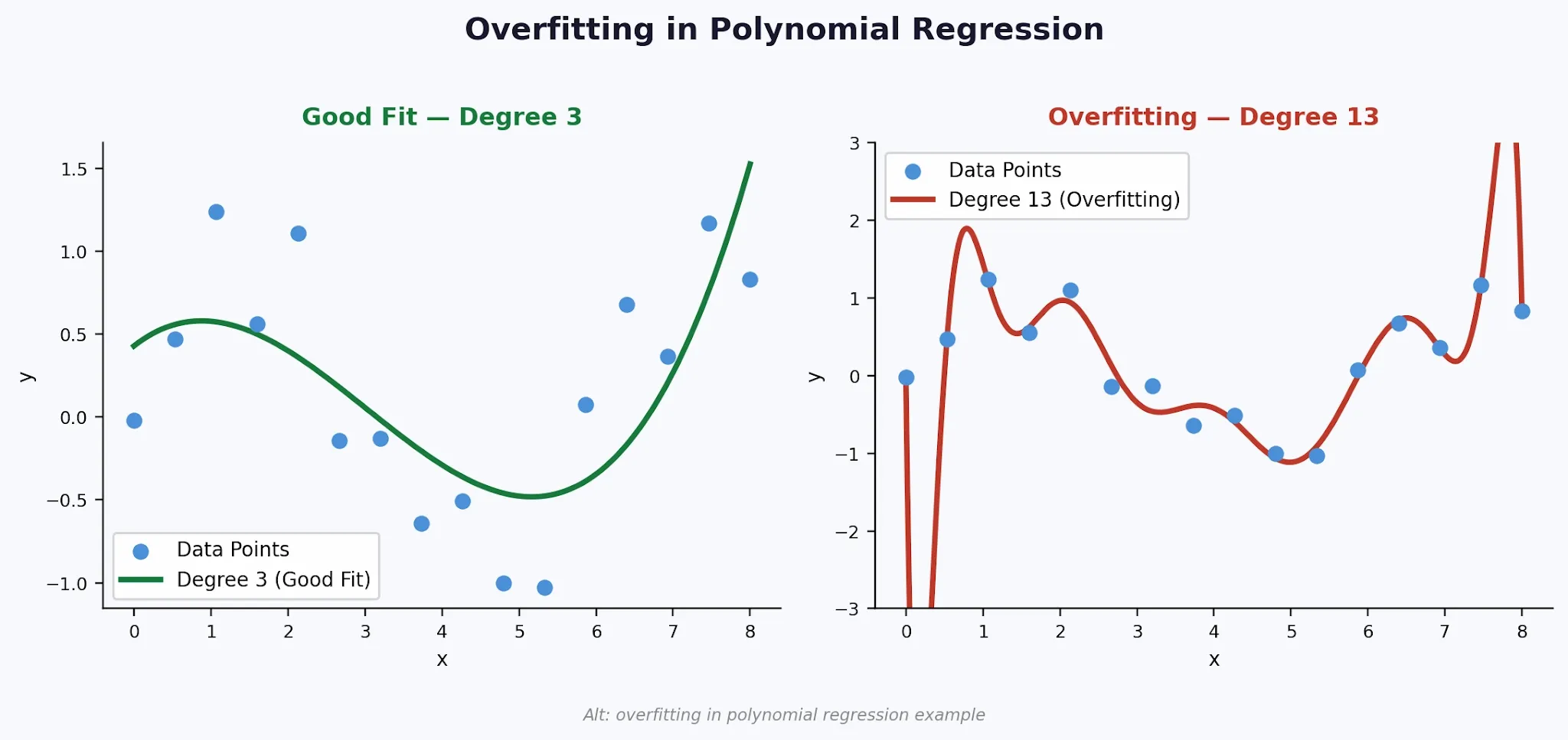
Overfitting in the case of Polynomial regression is one of the biggest risks. It happens when the model fits the correct training data too precisely. It also helps memorise all the data points and then fails to generalise it to any new data.
1. Why Overfitting Happens
A high-degree polynomial gains enough flexibility, and it actually passes through almost every training point. Real data contains random things where you can find multiple outputs. The model learns that random points are as if they were a true underlying pattern. This destroys its ability to predict the accurate aspect of unseen inputs.
2. Symptoms of Overfitting
Consider certain symptoms of overfitting.
- Very high accuracy on training data, but it has poor accuracy on test data
- Wildly oscillating multiple predictions between actual data points
- Model coefficients that shift dramatically with small changes to proper training data
3. How to Prevent Overfitting
To prevent overfitting, there are certain steps to consider.
- Start with a low degree and then increase only when underfitting is clearly evident
- Use the k-fold cross-validation that helps evaluate performance across multiple data splits
- Apply Ridge or Lasso regularisation to ensure constraints and penalise large coefficients
- Gather more training data when possible. This helps to train the model by reducing the model's sensitivity to multiple random things.
Bias-Variance Tradeoff in Polynomial Regression
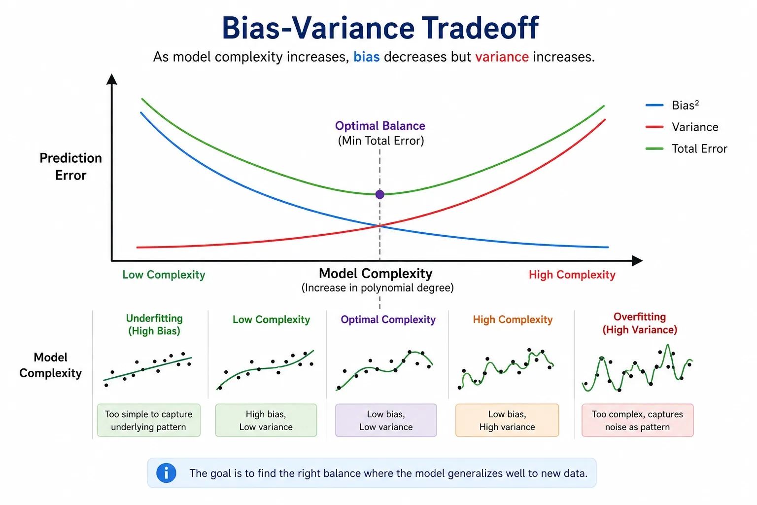
Polynomial regression explained in simple form to the concept of bias-variance tradeoff is actually a balancing act. It defines how to create the perfect balance between a model's simplicity and its complexity.
Low degree means high bias; the model is too simple and even misses real patterns. A high degree always means high variance, and the model is too sensitive to random things in the training data. This is where plot training vs. test error across different degree stages assists with cross-validation. It applies to find the optimal balance level.
Here, the total error is calculated as - Total Error = Bias² + Variance + Irreducible Error.
Also Read: Can You Do an MCA in AI & ML Without a Coding Background?
Advantages and Disadvantages of Polynomial Regression
As you already know about the polynomial regression definition machine learning, it’s time to have a clear idea on the advantages and drawbacks. Though the advantages of polynomial regression outweigh the drawbacks, take a look at both aspects.
| Advantages | Disadvantages |
|---|---|
| Captures non-linear trends accurately | Prone to overfitting at high degrees |
| Easy to implement with Python’s scikit-learn | Sensitive to multiple platforms while working with training data |
| Flexible and much more adjustable by changing the degree | Poor data accuracy beyond the training range |
| Definitely a better fit for curved real-world data than linear progression | Computationally heavier because of many features. So proper training of the model is necessary. |
Understanding these trade-offs realistically helps data analysts to develop accurate models and use the polynomial regression concept at its best to ensure the best outcome.
Evaluating Polynomial Regression Models
A polynomial regression model in machine learning must be evaluated based on certain performance metrics. These metrics help to ensure better outcomes.
1. R² Score
R² score stands for the coefficient of determination. It measures how much variance in the target variable the model explains. For example, a score of 1.0 is perfect, but scores above 0.85 on test data often indicate strong predictive performance.
2. Mean Squared Error (MSE)
MSE averages the squared differences between predicted and actual values. Lower is better. Squaring the errors penalises big mistakes more heavily than small ones.
3. Root Mean Squared Error (RMSE)
RMSE is the square root of MSE that shows the same units as the target variable. It is also easier to interpret than MSE. A large gap between training RMSE and test RMSE is a reliable sign of overfitting.
Real-World Applications of Polynomial Regression
Polynomial regression in machine learning is widely used across multiple industries because many business relationships are non-linear.
| Multiple Industries | How They Use It |
|---|---|
| Sales Forecasting | Business data analysts use polynomial regression to predict:
|
| Stock Market Trend Analysis | Financial analysts apply the concept of polynomial regression to model:
|
| Healthcare Analytics | Healthcare systems use the regression models for:
|
| Demand Forecasting | Retailers and supply chain companies use the concept of polynomial regression to estimate:
|
| Weather Modeling | Meteorology department and experts use the polynomial regression concept to analysis:
|
As the concept of AI adoption accelerates globally and across multiple sectors, predictive analytics continues to become more important in decision-making systems. According to the recent data from IBM Research Insights, 66% of enterprises reported AI-driven productivity improvements. This data reinforces the growing importance of machine learning models in multiple business operations.
Take the next step in your career ?
Conclusion
Organisations these days invest heavily in both AI and machine learning technologies. Hence, understanding the techniques and the fundamentals of polynomial regression in machine learning with their core concepts is increasingly valuable for aspiring professionals. Most candidates who want to start a career in this field or want to upskill themselves are looking for such courses.
Students and working professionals pursuing AI, data science, and machine learning courses, or professionals who want to earn expertise or upskill, can opt for courses offered by Amity Online. Gather the most practical, industry-oriented, and career-focused knowledge in multiple emerging technologies and continue a valuable career.
Check Out Our Top Online Degree Programs

Author
Similar Blogs
What is Copywriting? Skills, Salary & How to Start a Career
Artificial Intelligence Salary in India: Average & Well Paying Jobs
What Is a Scrum Master? Role, Salary, Certifications and Career Path (2026 Guide)
Apply Now
Similar Blogs
What is Copywriting? Skills, Salary & How to Start a Career
Artificial Intelligence Salary in India: Average & Well Paying Jobs
What Is a Scrum Master? Role, Salary, Certifications and Career Path (2026 Guide)
Apply Now
frequently asked questions
What is polynomial regression in machine learning?
+Polynomial regression in a machine learning model is used as an advanced algorithm. It shows non-linear relationships between variables. It fits a curved line and multiple data points by raising independent variables, converting a clear picture of the whole curve.
How does polynomial regression work?
+Polynomial regression in ML works on the input features into higher-order terms such as x² and x³. Then it applies the formula of linear regression on those transformed features and fits those into a curve through the training data.
What is the difference between linear regression and polynomial regression?
+Linear regression fits a straight line and works only for linearly related data. Polynomial regression fits a curve by applying higher-degree transformations. Hence, in the machine learning concept, it is widely accepted and ideal for non-linear data.
When should we use polynomial regression?
+If there is any nonlinear pattern in the residuals, then this might be an indication that polynomial regression could offer a better fit to the data. Polynomial regression works if the data shows a nonlinear and curvilinear relationship (like a U-shape or S-curve).
What are the advantages of polynomial regression?
+Polynomial regression excels at capturing complex, non-linear relationships and curvilinear patterns. These are something standard linear models miss. It offers high flexibility while maintaining analytical interpretability. This concept also requires low computational overhead.
What are the disadvantages or limitations of polynomial regression?
+There are certain limitations in polynomial regression. It is highly flexible for modelling non-linear data, but it can not deal with severe overfitting, extreme sensitivity to outliers, and parameter interpretability. If a model’s complexity increases, the algorithm becomes less stable.
What are polynomial features in machine learning?
+Polynomial features are a type of synthetic feature that is used in machine learning models by raising original features to higher powers. They are generated during preprocessing while allowing a linear regression model to fit polynomial curves to the data.
How is polynomial regression implemented in Python (or sklearn)?
+Polynomial regression is implemented in Python or Sklearn, a machine learning model. It helps to transform independent variables into polynomial terms and applies a linear regression model to those new features.
Where is polynomial regression used in real-life applications?
+Polynomial regression is used in some real-life applications. These include - #Epidemiology & Healthcare # Economics & Finance: # Climate & Environmental Science # Engineering & Physics